Stata Tips #12 - SVG graphics in Stata
Stata can now export any graphs to SVG. Scalable Vector Graphics (SVG) is a file format with a lot of advantages for Stata users. In this post, we will outline what makes SVG great, and why Stata is better at making SVG than other analysis packages. We'll also show you how you can manipulate SVG after you export it to great effect.
What is SVG?
Images can be stored digitally as raster files, which essentially list the colours of all the pixels. Generally, with formats like PNG and JPEG, there are compression algorithms that save space, so not every pixels is literally listed in an array (though that is the case for the old bitmap BMP file format).
The alternative is vector graphics, which instead contain a recipe which the computer can follow to recreate the image, by putting together elements like lines, rectangles, polygons, circles, colour gradients and so on. Because these files do not have information by the pixel, if you enlarge them, they do not become blurred or pixelated. You might have noticed this about PDFs before: no matter how much you zoom in on the text, it stays sharp-edged and clear.
The SVG can be converted to a raster later, at whatever size or resolution is required, which makes it an ideal standard format to use for saving and sharing your graphs. Save everything as Stata's own .gph, and as .svg, and you will have covered all your options.
SVG, PDF, and PostScript are the most common vector formats. SVG differs from the others in being written in plain text, which means humans can read and understand it, not just computers. That also means that humans can edit an SVG file, perhaps changing some text or the colour of a line.
Just as there are software packages to edit raster graphics, like Photoshop or GIMP, there are also editors for vector graphics, like Illustrator (a commercial package by Adobe) or Inkscape (an open-source package). With SVG, you have the option of editing it in one of these, or manually in a text editor. We'll expand on this idea below, and show why it is worth looking into, even if the idea of editing files by hand sounds scary.
How do you get an SVG file out of Stata?
graph export acquired the ability to export to SVG in Stata version 14, but it was somewhat experimental and wasn't documented in the manual or help files until version 15. However if you have 14 or 15, you can use it. Simply type:
graph export mygraph.svg
and Stata will do the rest for you. In version 15, you will find SVG in the menu as well:
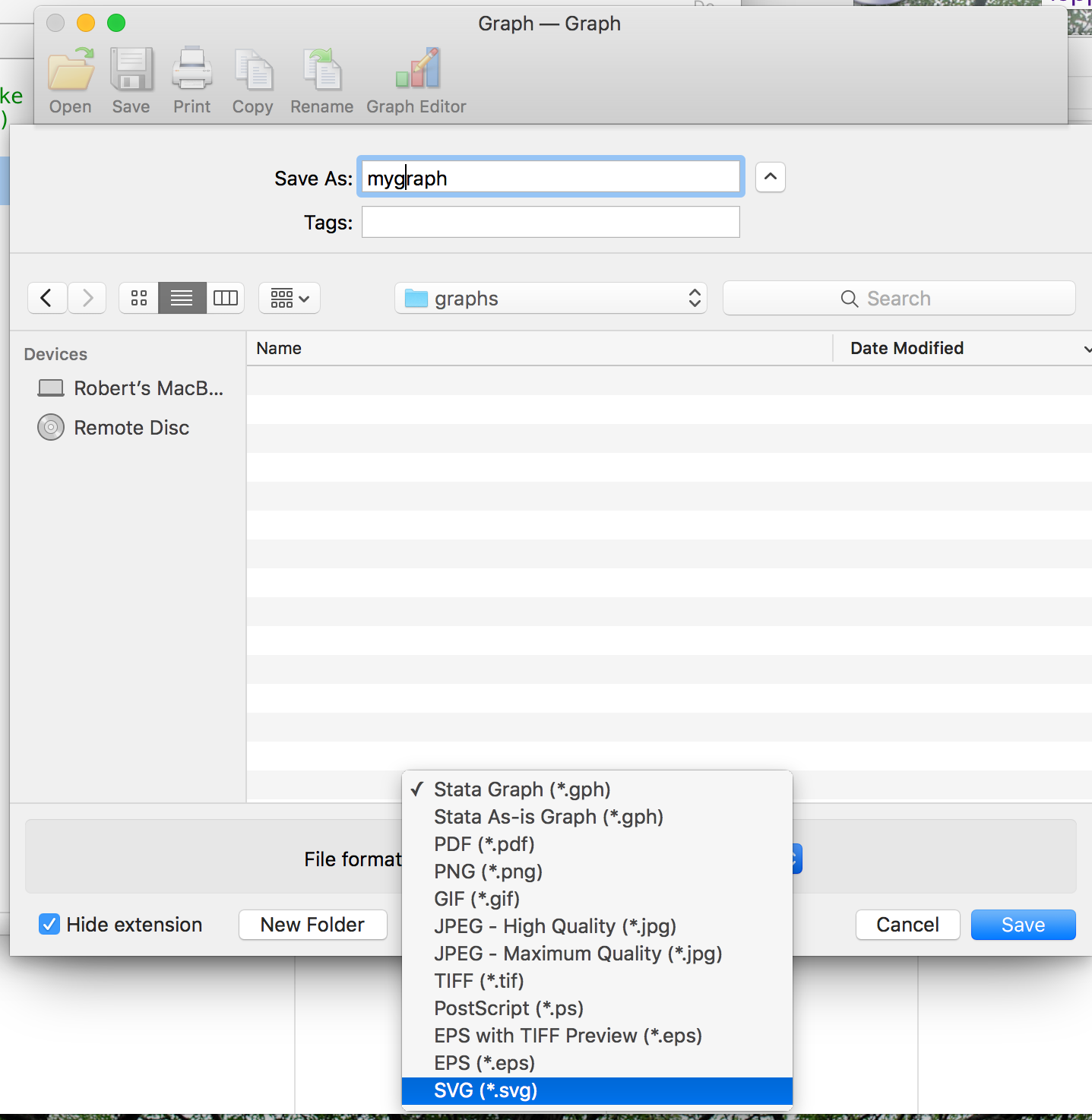
There are not many options to deal with if you use graph export from the command line or a do-file. You can change the size, which matters only in terms of the text in the graph, which will appear smaller as the whole of the image gets bigger. Because of vector graphics, there is no need to save a large version of your graph to display on a projector or to please a publisher.
Why Stata is especially good at SVG
SVG outputs are available in other analysis software, though not every package, but Stata's is particularly useful because it is lightweight and readable. In the event that you want to edit the SVG by hand, you will find that a Stata SVG file, opened in a text editor (Atom, in the case of these screen shots), looks like this:
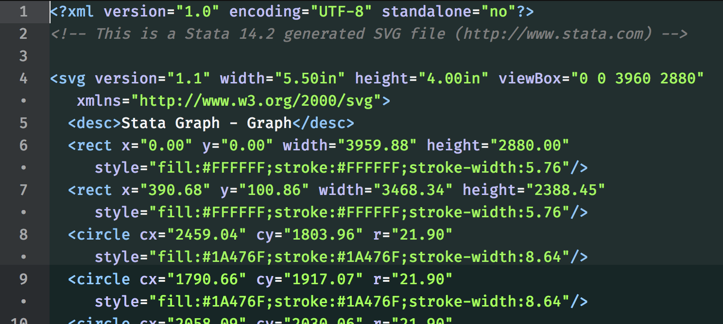
So, here you can see that there are circles and lines, which are obviously components of the scatter plot we made, which actually is just the sepal width versus sepal length from that much-loved dataset, Fisher's irises. It takes just 184 lines of SVG code to draw a scatterplot of those 150 observations.
This SVG syntax, where each object is inside less-than and greater-than brackets like this <rect>, is a special case of Extendable Markup Langauge (XML). Once you get a bit of practice at reading it, you will find it quite approacheable.
However, other data analysis software makes less approacheable, and more bloated, SVGs than Stata. Even the "svglite" package for R, which is supposed to reduce this bloating, doesn't achieve the same clarity. You can read more about the comparison in this blog post.
Adding transparency if you have Stata 14
Stata 15 introduces semi-transparency for graphics, which we discussed in a previous post. But if you have version 14, you can still export your graphs as SVG, and add the transparency there. I'll outline two ways to do this; bear in mind they are examples of how you can achieve different effects by editing the SVG code, and there are many more aspects of your graphs that can be tweaked beside these.
The first way to do this is to open up the SVG file in a text editor, find the colour you want to make semitransparent, and edit that colour with a find-and-replace. In the scatterplot code we saw above, there are rectangles (<rect ... >), which are the boundaries of the plot region, the background for the graph region, and so on, and there are also circles (<circle ... >), which are the markers for the data. The circles include colour codes like this: (style="fill:#1A476F";stroke:#1A476F).
SVG uses RGB (red, green, blue) coordinates to define colours, and each of those constituent primary colours can take a value from 0 to 255. Those values are recoded in hexadecimal, so they go from 00 to FF. 1A476F is Stata's "navy". You can see from the code that it is mostly blue (6F), with some green (47) but very little red (1A), and none of those are very high values, so it is quite dark. Actually, you can extend RGB to what is called RGBA, adding an "alpha" value on the end, which controls the opacity. 1A476FFF will be completely opaque, just the same as 1A476F, and 1A476F00 will be completely transparent (invisible).
So, to make the markers 50% transparent, all you need to do is to find 1A476F and replace it with 1A476F80. That's easy to do in any text editor. But what if there are other parts of the graph in navy, which you don't want to be semi-transparent? Just export your graph with the markers, or lines, or whatever you want to change in a different colour to everything else, then find that and change it to semi-transparent navy.
The second way to do this is within Stata with the filefilter command. If you know what the RGB code is, you can get it found-and-replaced without having to mess around in text editors -- very helpful if you have multiple graph files to edit. filefilter might work like this:
filefilter oldgraph.svg newgraph.svg, from("#1A476F") to("#1A476F80")
That will create a new SVG file with 50% transparent navy markers.
Editing in Inkscape or Illustrator
Apart from the tweaks that can be done in a text editor, more complex changes can be made in vector graphics editing packages like Inkscape or Illustrator. There are so many ways you could use this, it's impossible to do justice to it in this post, but to give an example, you can isolate a region of a line and give it a visual effect like this neon glow:

That is purely made out of SVG components, but it would be tedious to add it in the text editor. You can also move objects very easily, perhaps to superimpose graphs in a way that can't be done inside Stata, and you can easily add and align annotations.
What else can SVG do?
Having your graphs in SVG opens the door to interactivity. Because SVG is a form of XML code, it can be placed inside the HTML file of a web page, and can be manipulated using the web language JavaScript. Once you have the SVG file in a page with sliders, buttons and other controls, the reader can start to manipulate it. If you want to find out more about this, look into the JavaScript library called D3 (Data-Driven Documents).
Like the neon effect above, SVG includes gradients of colour and other visual effects, and animation can be added in various ways. I recommend the talks online by Sarah Drasner (who also has an excellent book on the subject of animating SVG) and Nadieh Bremer, if you want to find out more.