
Stata Tips #8 - Spatial Analysis in Stata 15
One of the new features in Stata 15 is spatial autoregressive models. These account for correlation between points or areas in space in the same way that time series models include correlation over time. To work with these, we typically have some data where each observation belongs to a point or area in space, and then more data files that define the shapes and positions of those points or areas.
There are three ways to go about defining the shapes and positions. Firstly, you can feed in shapefiles, which are a very widely used standard in geographic data, defining the boundaries and names of regions such as countries. Secondly, you can supply co-ordinates that pin-point each observation on a map. Thirdly, you can work without any location data but just specifying a matrix of how much one observation is believed to influence or be influenced by another.
Data in a social network can also be analysed with this third approach: instead of physical proximity defining the correlations, it is links between one person or organisation and another.
Let’s start with a fairly simple example, looking at carbon dioxide emissions and the relationship with socio-economic deprivation. Official statistics on carbon dioxide emissions can be obtained online; we retained the 2014 data only for this (and deleted the rows that give regional totals) to produce this file LA-CO2-2014.dta. We’ll also use the Index of Multiple Deprivation (IMD), which is a simple measure combining some information from the UK Census.
The United Kingdom is divided up into local authorities: regions with their own local government functions. Some of these relate to traditional counties, others to cities or towns. We can download a shapefile for local authorities here (actually Northern Ireland is not included in this, but just to keep the example simple, we’ll work with the rest of the country). Shapefiles often come in one .zip compressed file, which contains several files with all the data you need. In Stata 15, we can unzip the contents either using the command:
unzipfile "Local_Authority_Districts_December_2016_Full_Clipped_Boundaries_in_Great_Britain.zip"
or through the menu – all the spatial functions are found under Statistics: Spatial Autoregressive Models:

The menu brings up a dialog box with five stages, the first being “Setup”.
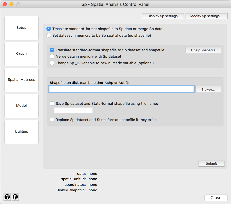
The “Unzip shapefile” button on the right will open up the .zip file. It contains six files, and it is best not to rename or move them as they will be used in what follows.
Our next step is to convert the shapefile to a Stata format. On the command line or do-file we would type:
spshape2dta Local_Authority_Districts_December_2016_Full_Clipped_Boundaries_in_Great_Britain
or in the menu, we select “Translate standard-format shapefile to Sp dataset and shapefile”, then browse for the “shapefile on disk”, selecting the newly unzipped file that ends .shp, then click on submit.
Either way, Stata will read all the shapefile data and construct two .dta files. One of these is much larger and called Local_Authority … _shp.dta – this contains the details of the boundaries and locations, and we should leave it alone. The other, Local_Authority … Britain.dta, contains a variable called lad16cd, which is a standard government code, and we’ll use this to link the carbon dioxide data to the shapefile data. We open this second smaller file, encode the lad16cd variable as a numeric variable called lacode (encode lad16cd, generate(lacode)) and then declare it to be spatial data using the command:
spset lacode, modify replace
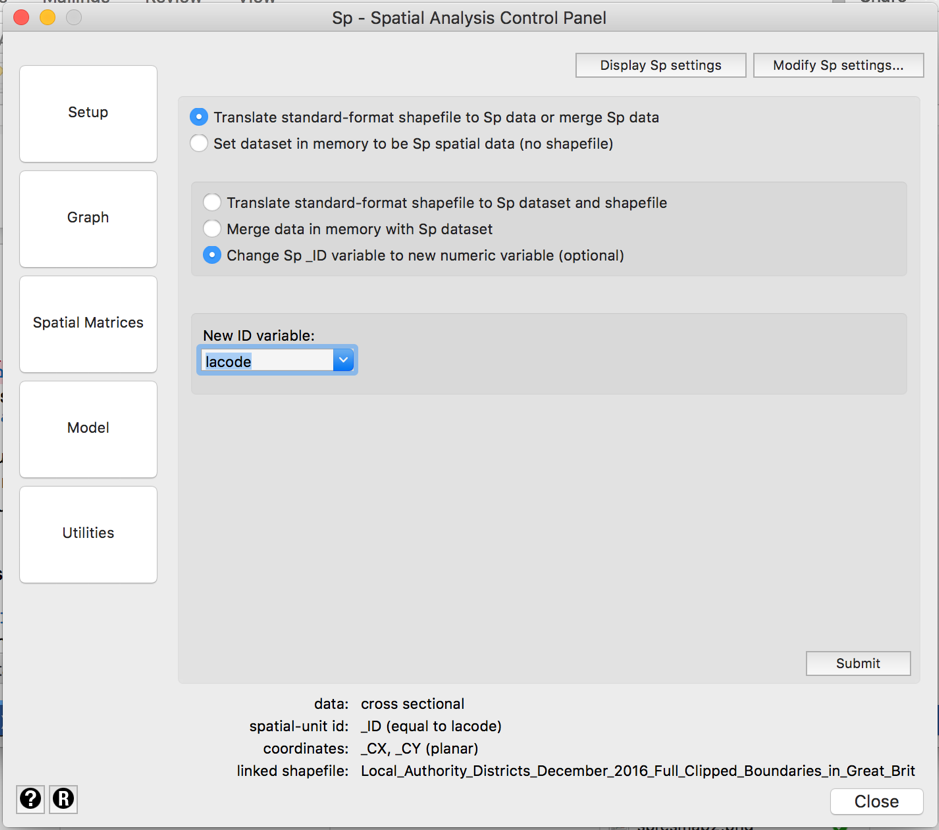
To do spset in the menu, we would click on Setup, then “Change Sp _ID variable to new numeric variable (optional)”. In the “ID variable:” drop-down list, scroll down to and select lacode, then click on Submit. A box will open with a question about replacing data; click on OK.
Now, we are ready to merge this shape data with our carbon dioxide data. On the command line:
merge 1:1 lad16cd using "LA-CO2-2014.dta"
or in the menus under Data – Combine datasets – Merge two datasets:
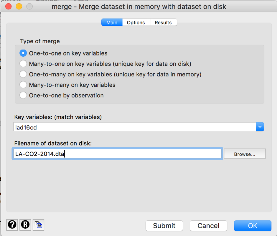
There are 380 local authorities matched, and 26 that occur only in the carbon dioxide data (these make up Northern Ireland, as mentioned above). We can just keep those with _merge==3.
keep if _merge==3

drop _merge
If we look at this data file, it just contains the carbon dioxide data that we started with, plus three variables _ID, _CX and _CY. These link to the …shp.dta file and so they should be left unchanged.
At this point, we can draw a choropleth map of the domestic CO2 emissions in thousands of metric tons by simply typing:
grmap domestictotal
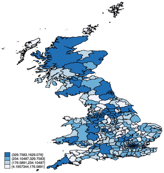
grmap is a command contributed by the user community, and there is no menu for it in Stata. You can find and install it by typing findit grmap. We can improve the look with several useful options which we will return to later.
Looking at this, there appears to be some regional clusters where emissions are higher, which suggests autocorrelation. Some of this, however, will be due to population, because the carbon dioxide data is in total thousands of tons.
We can merge in the deprivation data too:
import excel /// "File_10_ID2015_Local_Authority_District_Summaries.xlsx" /// , sheet("IMD") firstrow clear

keep LocalAuthorityDistrictcode2 IMDAveragescore

rename LocalAuthorityDistrictcode2 lad16cd

merge 1:1 lad16cd using "CO2-merged.dta"

keep if _merge==3

drop _merge
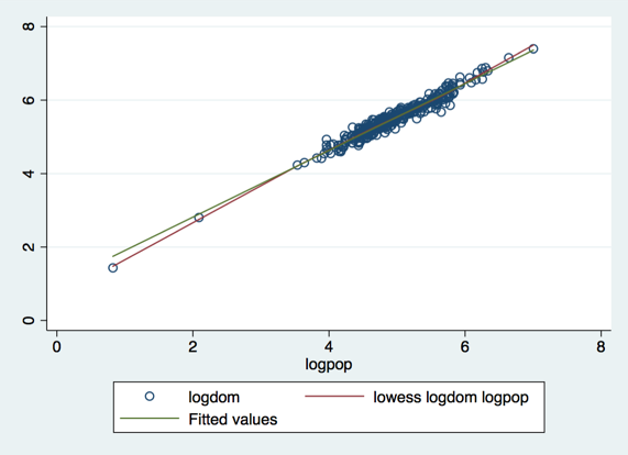
The values in the domestictotal variable are quite skewed and a simple regression plot against IMD shows heteroscedasticity (the scatter above and below the line of best fit increases as the values increase); we can fix this by taking logarithms of the domestictotal. We can then see that log-domestictotal and log-population are very strongly correlated, as we might expect: more people emit more carbon dioxide. The two very small local authorities are the Isles Of Scilly and the City Of London. They are a familiar headache to British statisticians because of their unusually small populations, and are sometimes omitted from analyses, though here there is no reason to do so.
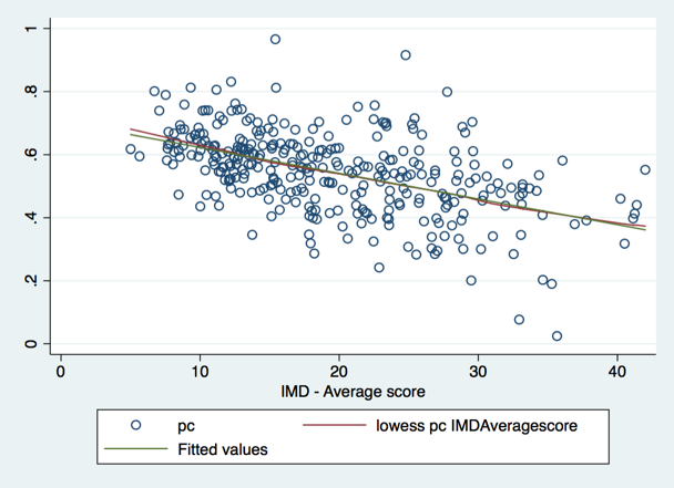
We can also fix the population differences by calculating a per capita dependent variable by dividing the domestictotal variable by the population variable, and then taking logarithms (or equivalently, subtracting the log-population from the log-domestictotal). Then, we can run a regression that predicts log-per-capita emissions based on IMD, and accounts for spatial autocorrelation. A scatterplot of log-per-capita emissions versus IMD shows a negative slope that, compared with a LOWESS smoother curve, is very close to a straight line.
Let’s think about the modeling choices. SAR models can have correlation in the dependent variable, or the independent variable(s), or the error terms. If we apply it to the dependent variable, we are saying that a region could have high emissions just because the neighbouring region does too. This makes sense if we think there are regional factors at play, such as types of housing, climate, availability of different forms of energy, or cultural differences.
If we apply it to the independent variable, IMD, we are saying that the regional correlation seen in the map is down to nearby regions sharing high or low levels of deprivation. It’s worth understanding what this IMD number really reflects (and doesn’t reflect). It is a weighted average of official statistics on these topics (weights in parenthesis):
- Income Deprivation (22.5%)
- Employment Deprivation (22.5%)
- Education, Skills and Training Deprivation (13.5%)
- Health Deprivation and Disability (13.5%)
- Crime (9.3%)
- Barriers to Housing and Services (9.3%)
- Living Environment Deprivation (9.3%)
Although there are some regional trends in deprivation, there are also adjoining local authorities where one is affluent and the other poor, especially in urban areas, so this does not seem so well justified.
If we apply it to the error terms, we are effectively saying that, after adjusting for IMD, there are regional clusters of similar residuals, which probably indicates that there are spatially correlated determinants of emissions which we do not have to hand, or understand, and which are not associated with IMD. Although this might well be true, the first option of correlation in the dependent variable seems most interesting and plausible.
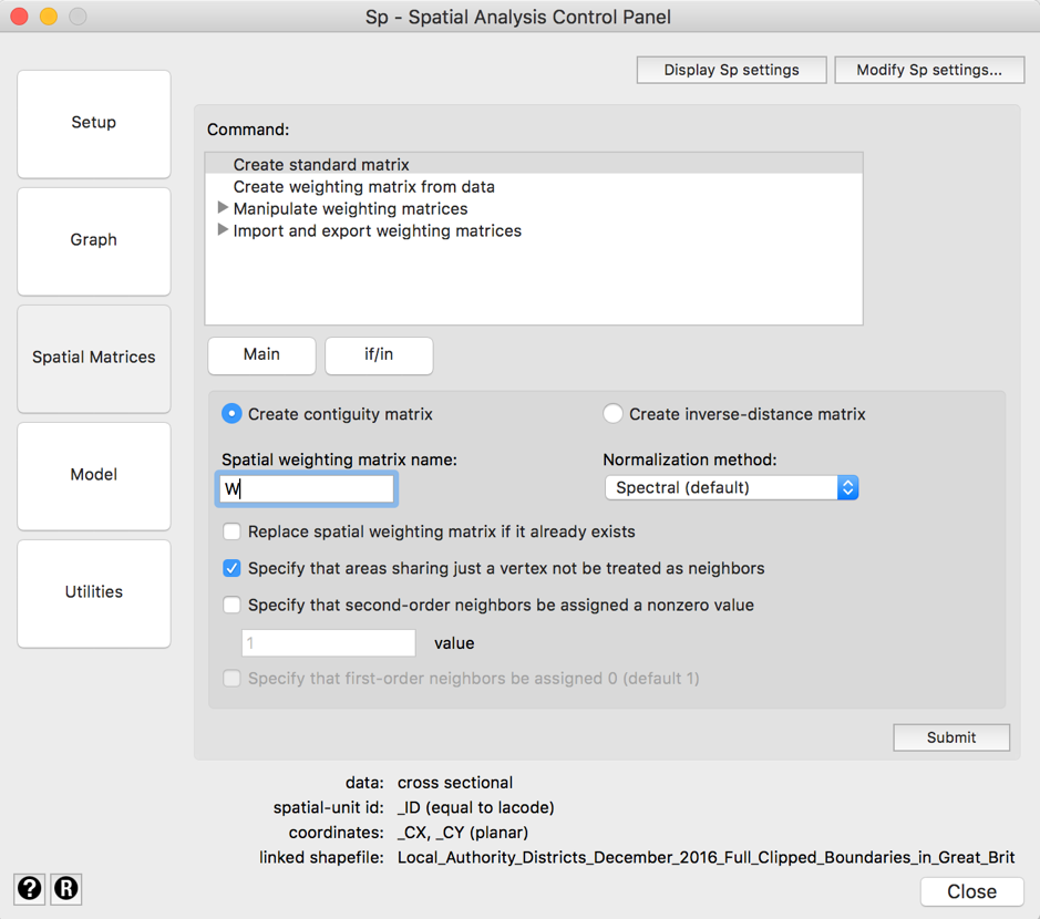
Next, we have to choose from two types of correlation matrix. We can also specify one ourselves, but the spmatrix command will easy make them for us. The first choice is that bordering local authorities can influence one another, but no others. This is sometimes called an adjacency matrix or contiguity matrix (Stata uses the latter term). The second choice is to have the correlation proportionate to the inverse distance, which uses the shapefile variables _CX and _CY to calculate distances between local authority midpoints. We’ll try both and compare them.
We can type:
spmatrix create contiguity W, rook

spmatrix create idistance W2
Or in the menu, click on “Spatial Matrices”. Below “Command:”, select “Create Standard matrix”, click on “Main” and select the type of matrix before clicking on “Submit”.
Then, we are ready to go ahead and fit the regression models. Simply running a linear regression without any spatial information gives us a baseline to compare our models to. We can type:
regress pc IMDAveragescore

predict regres, residuals
This gives a slope of -0.0082 (95% confidence interval -0.0066 to -0.0097, p<0.001), relating IMD to log-per-capita emissions: areas with higher deprivation have lower domestic emissions. Then, we can look at the residuals, scattered against the untransformed emissions, and draw the residuals on a map:
scatter regres domest, msymbol(Oh) name(regres, replace)

grmap regres, clnumber(9) fcolor(BuYlRd) ///

name(regresmap, replace)
Now, we bring in some of the options for grmap. We ask for the variable regres to be cut into 9 categories, and we apply a color scale called BuYlRd to it. This has 9 categories, and is called a diverging scale because there is a pale yellow in the middle around residuals of zero (perfect fit to the data), with darker blue indicating large negative residuals (the model over-estimates the data) and darker red indicating large positive residuals (the models under-estimates the data). This is one of several useful color scales devised by Cynthia Brewer, which you can learn about at www.colorbrewer2.org. The legend could be made neater too.
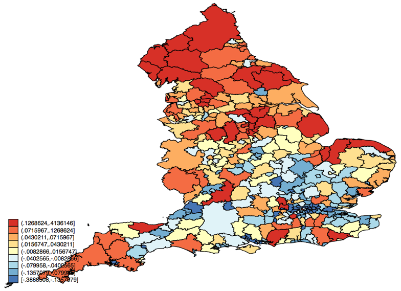
This is immediately a good case for a spatial model because the residuals are geographically clustered. There are some large regions of reds and blues. Thinking about what they might tell us, the blue region around London suggests that, despite deprivation levels that are quite high in some authorities and low in others, domestic carbon dioxide emissions are lower than expected throughout, while the opposite is true of local authorities at the Northern edge of England, in Cumbria and Northumberland.
To get the SAR model with the contiguity matrix, we can type:
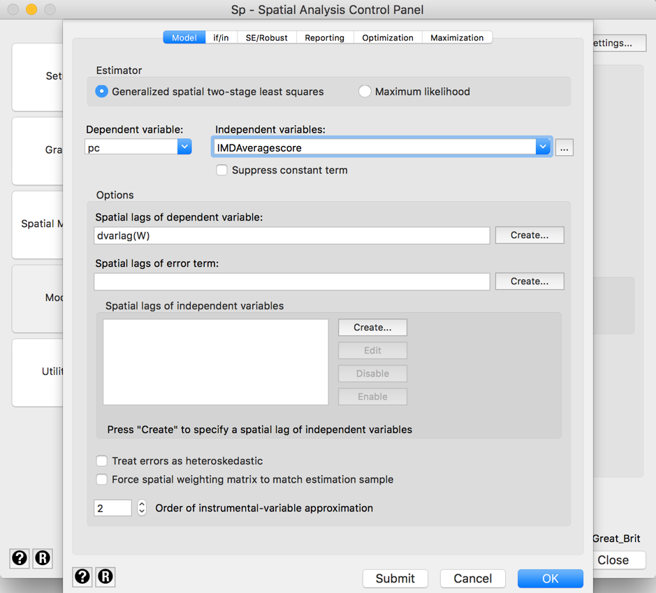
spregress pc IMDAveragescore, gs2sls dvarlag(W)
The dvarlag option indicates the correlation or lag applied to the dependent variable, using the matrix called W that we made earlier. The gs2sls option is one of two algorithms to fit these rather challenging models, and you can read more about this in the Stata Spatial Manual.
In the menus, we would click on “Model”, select “Spatial autoregressive models”, click on “Go -->”, and select “Generalized spatial two-stage least squares”. Open the drop-down list for “Dependent variable:” and scroll until you see the pc variable; click on it. Do the same for “Independent variables:” and select the variable IMDAveragescore. To the right of “Spatial lags of dependent variable”, click on “Create...”, then choose “W” from the drop-down list for “Spatial weighting matrix”. Click on “OK” and the model will be fitted.
We can do the same model, but with the inverse-distance correlation matrix. The contiguity matrix model has slope -0.0063 (95% confidence interval -0.0047 to -0.0078, z = -7.7, pseudo-R2 0.29) , while the inverse-distance matrix model has -0.0085 (95% confidence interval -0.0071 to -0.0099, z = -11.7, pseudo-R2 0.37). If we generate the choropleth maps of residuals as before, we get these:
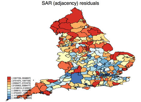
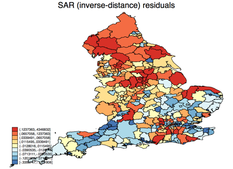
Which type of correlation matrix is correct? The pseudo-R2 suggests that the inverse-distance matrix fits the data better, but the answer really depends on your understanding of the context of the data and the question we are trying to answer. Local authorities in the UK have very different sizes, so it is possible for two to be separated by another, and therefore non-contiguous, but very close together geographically, especially in urban areas. Very large, sparsely populated rural areas might have the opposite difference: contiguous but a long distance between the centres. We can see the inverse-distance matrix working better for the large rural areas which are red and under-estimated by the contiguity matrix model, and breaking up the pocket of blue over-estimated local authorities in London and environs (the small regions in the south-east). On the other hand, a new pocket of red has formed around Sheffield, slightly north of centre. To really critique these further, we would need more data about the reasons for higher or lower than expected emissions.