Stata Tips #21 - Stata 15's new survival analysis with interval-censored event times
Stata 15's new survival analysis with interval-censored event times
What is it for?
Often, time-to-event or survival data are gathered at particular observation times. A physician will detect the recurrence of cancer only when there is a follow-up appointment, and a biologist might know that a study animal in the wild has died when they visit the site, but not exactly when it happened. In either case, all we know is that the even happened between the two appointments or visits, which is to say that there is a lower limit and an upper limit to the survival time. In statistical parlance, data like this are interval-censored.
Stata version 15 includes a new command, stintreg, which provides you with the familiar streg parametric survival regressions, while allowing for interval-censored data. Just by typing estat sbcusum, you obtain test statistics, critical values at 1, 5 and 10 percent, and a cumulative sum (CUSUM) plot, which shows when, and in what way, the assumption is broken if it is.
An example with medical follow-up data
In this post, we'll apply stintreg to a dataset from David Collett's textbook, "Modelling Survival Data in Medical Research" (3rd edition) (Example 9.4). This is from a real-life study that examined breast retraction, a side-effect of breast cancer treatment, and compared women treated with radiotherapy alone and those treated with radiotherapy and chemotherapy. You can download the data in CSV form here and follow along with this do-file.
There are three variables: treatment group, start time of the interval (the last appointment at which there was no sign of retraction) and end time of the interval (the first appointment where there was retraction). First, let's visualise the dataset. Time is on the vertical axis, and the women are ranked by start time from left to right, in the two treatment groups. The exact time when retraction appeared is somewhere in the grey lines. Ideally, we would see a lower risk of retraction as grey lines stretching off to the top of the chart without red dots, and high risk indicated by red dots low down in the chart. But, it is hard to judge whether there are any differences.

Let's fit some streg models, using naive approximations of the data so that they look like they are exactly known. First, we use the start time (the last retraction-free appointment).
gen naive = (end!=.)
stset start, failure(naive)
streg treatment, distribution(weibull)

This shows a very strong and statistically significant detrimental effect of chemotherapy. Next, we use the mid-point between the two appointments:
gen naivetime = (start+end)/2
stset naivetime, failure(naive)
streg treatment, distribution(weibull)
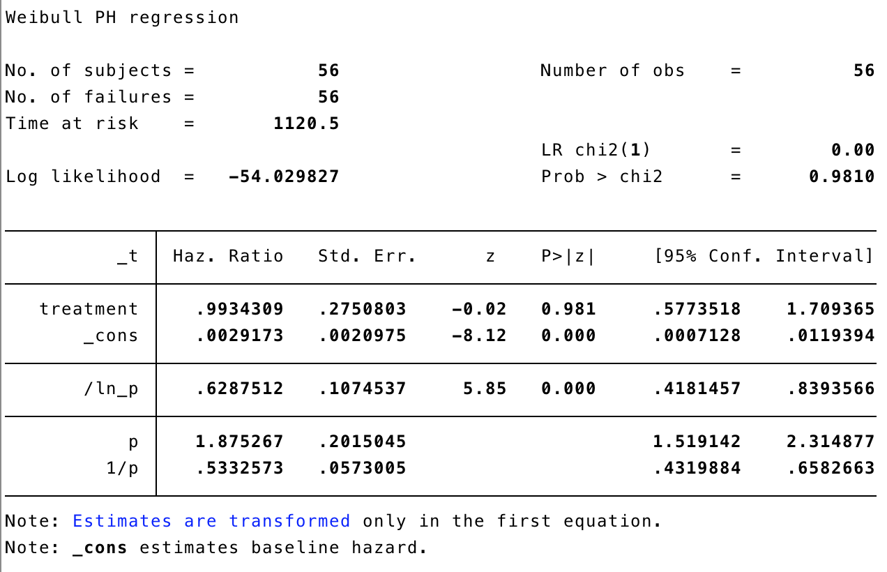
Oh dear! This shows an almost non-existent difference between the two groups, with no statistical significance. Which can we trust? We need to account for the interval censoring ina principled way, as part of the overall probabilistic model for the data, and this is where stintreg comes in.
stintreg treatment, interval(start end) distribution(weibull)

Now, we can see that the treatment group difference is quite large, and quite compelling in terms of significance. Note that, because the models are very different, we can't compare the log-likelihoods.
Why does this matter?
Interval-censored data are everywhere. Being able to account for the uncertainty in the data gives more honest answers, not only by avoiding bias but by having the right level of uncertainty. If you fill in the "blank" with a single number, then you give Stata the false impression that the data are exactly known, and the inferences (p-values, confidence intervals) that follow will be falsely precise as a result.