Can Economists Forecast the Future?
Written by Jennifer L. Castle and David F. Hendry.
We all forecast many things every day, probably unconsciously, but forecast errors can be very expensive. For example, large forecast errors of COVID-19 cases may lead to a shortage of ICU capacity. Good forecasting pays handsome dividends, but it is riddled with difficulties. Forecasts typically go very wrong when there are sudden changes or unexpected shifts in the data. This could be due to numerous factors including external events such as wars, pandemics or climate crises, changing policy, or changing behaviour.
This blog is aimed at economists and applied econometricians who work with time-series data and want to understand when forecasts are likely to be accurate or not, and how to avoid systematic errors. In this short piece we describe how to forecast following a break. This can be done very easily in OxMetrics which provides the state of the art in forecasting methodology.
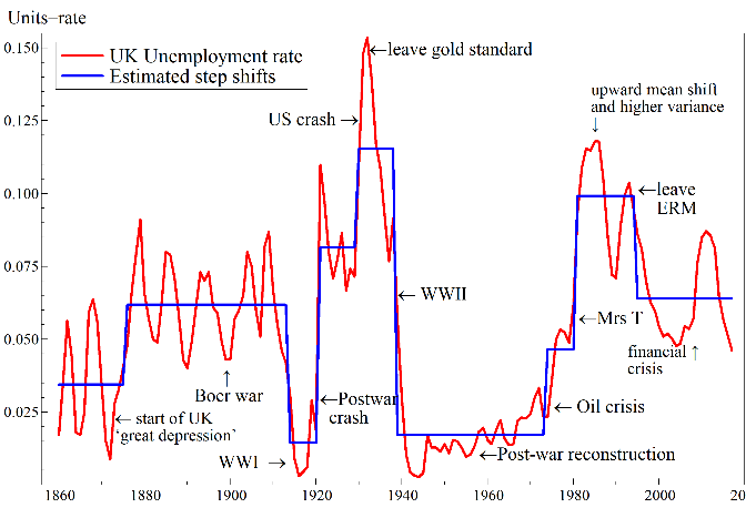
First, you may ask why are we concerned with breaks in the data? The figures below show more than a century and a half of data for UK wage and price inflation in the left panel, and the UK unemployment rate in the right panel. There are a huge number of location shifts and outliers in data. Imagine standing just prior to one of these big jumps – could you forecast the sudden shift? History shows us that this is unlikely, as most of these shifts were unanticipated based on information available at the time.

But what about forecasting just after a big shift – could you avoid persistently large forecast errors? The evidence is surprisingly poor for economic forecasts. The figures below show the prevalence of forecast failure. On the left, we have the UK Office for Budget Responsibility forecasts for productivity, and on the right we have the ECB core inflation forecasts. These make systematic forecast errors for long periods after a location shift in the data. We call these hedgehog graphs for obvious reasons, and you can look in almost any forecast domain and find examples of these hedgehog graphs. Not only that, you can produce them yourselves in OxMetrics; under forecast options select hedgehog plots and see if your forecasts suffer the same fate as those of many professional forecasters.


So how do we avoid systematic forecast failure? First we need to understand why it occurs, and then adapt our forecasting models to make them robust to persistent forecast errors. Most forecasting models belong to the huge class of equilibrium-correction models that have fixed equilibrium states to which the model tends to converge. The class comprises most widely-used models, from regressions, scalar and vector autoregressions, through cointegrated systems, to volatility models like ARCH and GARCH. When the equilibrium does shift (which from the inflation and unemployment figures can be seen to occur often) the distribution of the variable has changed relative to its past behaviour, but the forecasting model has not. The model still thinks that the data are drawn from the previous distribution, leading to forecasts that try and converge back to the previous equilibrium. Unless the equilibrium is updated to the new location, systematic mis-forecasting will occur. This results in the hedgehog graphs seen above.
So how do we adapt our forecasting models to account for these shifts? Unless we somehow `know’ the new equilibrium, which is unlikely, the equilibrium convergence must be removed from the forecasting model. This can be done in a number of ways, but one such way, included in OxMetrics, is to robustify the forecasts by differencing out the equilibrium mean or growth rate while keeping the economic content of the forecasting model. When the equilibrium first shifts, you will make a forecast error. But after the shift, the robust forecasting model will not be pulling the forecasts back to the previous equilibrium. The figure below shows UK GDP growth over the Great Recession in panel (a). The 1-quarter ahead forecasts using an equilibrium-correction model (EqCM) are given in panel (b) with ±2 standard error bands – the forecasts miss both the huge downturn and subsequent upswing. Panel (c) records the robust forecasts based on the same model. Despite some overshooting at the turning points, the forecasts are much closer to the outturns. Panel (d) records the squared forecast errors, highlighting the substantial benefits of robustification.

There are costs to using robust forecasts – there are few free lunches in economics. The forecasts have a larger degree of uncertainty so the trade-off for a reduction in bias is an increase in variance. But the benefits are substantial just after a break has occurred. So it can be thought of as an insurance policy – if the robust forecast differs significantly from your model based forecasts you might want to investigate whether there has been a break in the data. And it has never been so easy to do using OxMetrics; just select the option to ‘include robust forecasts’ and a graph will appear with both your model based forecasts and the robustified forecasts. Now you can avoid hedgehog graphs for good!
Jennifer L. Castle and David F. Hendry are both professors at the University of Oxford and run Climate Econometrics ,where you can find out the latest news of their research and publications. Gain further insight into how to forecast the future, joining Jennifer L Castle, David F. Hendry and Jurgen A. Doornik for their 'Climate Econometrics Spring School' 15-17th March 2021.
The course provides an introduction to the theory and practice of econometric modelling climate variables in a non-stationary world. It covers the modelling methodology, implementation, practice and evaluation of climate economic models. We hope to see you there!